Fast and accurate location of problem events at regional distances is among the key tasks of seismic nuclear test monitoring. In the current practice, such location is attained through construction of regional travel-time correction surfaces (source-specific station corrections, SSSCs) for the existing and proposed stations participating in seismic monitoring. SSSC corrections are obtained through prediction of the regional travel times followed by some kind of spatial interpolation (e.g., kriging) of the travel times measured from well-located “ground truth” (GT) events (Myers and Schultz, 2000). Where recordings of regional GT events are too sparse for meaningful interpolation, travel-time calibration is performed in terms of characterization of the propagation of seismic phases within the region of interest. Such characterization is performed either by associating the types of crustal and mantle tectonics with their corresponding travel-time patterns (Tralli and Johnson, 1986) that are further combined using empirical rules (Bondá́r and Ryaboy, 1997; Yang et al., 2001) or by building 3D velocity models (Villaseñor, 2001; Priestley et al., 2002).
In northern Eurasia, which is a focus area of seismic nuclear test monitoring, the first of these approaches is practically impossible without special calibration explosions. This vast area is largely aseismic, very few GT events are available, and station coverage is sparse. However, owing to the extensive program of lithospheric seismic studies (Deep Seismic Sounding, DSS) carried out in the former Soviet Union in the 1960s through the 1980s, this area is also among the world’s best covered with controlled-source, refraction-reflection profiling. A dense network of DSS projects traversed most of the territory of the Soviet Union and included a grid of regional-scale profiles that recorded Peaceful Nuclear Explosions (PNEs), several nuclear tests at Semipalatinsk and Novaya Zemlya test sites, and hundreds of chemical explosions (Fig. 42). Digital seismic data from several of these profiles have recently become available and provide unparalleled data sets for seismic calibration of northern Eurasia.
DSS/PNE data have been extensively studied for mantle velocity and attenuation structure (Yegorkin and Pavlenkova, 1981; Mechie et al., 1993; Pavlenkova, 1996; Morozov et al., 1998b; Morozova et al., 1999; Nielsen et al., 1999) and mantle and crustal scattering (Ryberg et al., 1995; Morozov et al., 1998a; Morozov and Smithson, 2000; Morozov, 2001; Nielsen et al., 2003; Nielsen and Thybo, 2003). Here, we present an application of DSS data to travel-time calibration of northern Eurasia by using a new seismic calibration technique inspired by the good aerial coverage, density, and continuity of the data sets. Controlled source recording offered unique opportunities for characterization of the lithospheric structures across the key tectonic boundaries and also for continuous observations of seismic events propagating across 0-3000 km ranges. PNE energy (mb >5) and spatial sampling density (10–20 km) were sufficient for consistent recording of the arrivals, capturing the detailed travel-time variations caused by the regional and local crustal structures (Figs. 43-45).
Although significantly denser and more continuous than most data sets available to calibration seismology (Figs. 42-45), DSS profiles are still far from the coverage required for a sufficiently detailed, 3D velocity modeling. In particular, owing to the nonuniqueness of 1D refraction travel-time inversion (Healy, 1963; Morozov, 2004), large and uncontrollable velocity-depth uncertainties would always remain in the resulting models. Fortunately, most of these uncertainties have little impact on the travel times; therefore, in the context of seismic calibration, an appealing approach would consist in cataloging the observed travel-time patterns directly, without attempting to mitigate the uncertainties of velocity inversion or resorting to associations of travel-time dependencies with tectonic types. Such cataloging could incorporate the key physics of the model-based approaches and also result in 3D velocity models (however, with the difference of their being the apparent velocity models).
The existing empirical travel-time calibration method is based on regionalization, that is, subdividing the area of interest into several regions, each of which is associated with the corresponding travel-time versus offset dependence. For sources and receivers located in different regions, the regional travel-time dependencies are combined by using a heuristic interpolation rule (Bondár and North,1999; Bondár et al., 2001; Yang et al., 2001), such as:

where S and R represent the source and receiver (both assumed to be located close to the surface), Li is the length of the great-arc segment connecting S and R and lying within the ith region, and dSR = ∑iLi is the total source-receiver distance. The regions are outlined based on their tectonic types, and several regionalization schemes have been proposed for northern Eurasia (Kirichenko and Kraev, 2000; Conrad et al., 2001).
Although equation (1) is convenient for interpolation, it is not based on the physical principles of body-wave propagation through the crust and mantle. Travel times at all offsets are interpolated as if the corresponding seismic phases were propagating along the surface and at a constant velocity. Dense DSS travel times (Fig. 46) illustrate a typical problem of assigning fixed travel-time patterns to large areas in this method. The regions are far too large to account for the crustal variability and, yet, too small to allow a meaningful description of the seismic phases propagating within the mantle. Assigning a single shallow structure to large areas appears to be a conceptual limitation insurmountable in this regionalization/interpolation approach. However, crustal structures are known to both exhibit the greatest variability and to have the strongest impact on the travel times (this has also been well documented in DSS interpretations; e.g., Morozova et al., 1999). Subdividing the regions into smaller blocks does not alleviate the problem because, with smaller regions, the edge effects caused by the ray paths crossing region boundaries become more pronounced.
The scale-length disparity could be resolved by abandoning the fixed region boundaries and making the travel-time interpolation (1) dependent on the offsets or, equivalently, ray parameters. Such interpolation would be based on the diving-wave kinematics and, thereby, reflect the vertical stratification and variable scale lengths of the lithosphere. Travel-time mapping would be more detailed at the near offsets corresponding to the shallow velocity structures where the variability is predominant. At progressively greater offsets, the model would lose detail because of decreased data coverage, greater path averaging, and also lower-velocity heterogeneity within the mantle. Another desirable requirement for any travel-time calibration model is that, in sparsely-sampled areas, the predicted travel times should approach the nearest available regional readings rather than be controlled by some “reference” curve based on global averages (as it is commonly done with the International Association of Seismology and Physics of the Earth’s Interior [IASPEI 91] model in existing methods).
Next, we describe a practical travel-time interpolation scheme implementing the preceding principles. When applied to regionalized models, this approach could be viewed as a more physical (i.e., employing diving-ray kinematics) alternative to the interpolation method (1); at the same time, the method does not require classification of the travel-time patterns and, similarly to tomography, it could be applied to large data sets with complex spatial data distributions. By contrast to 3D velocity modeling, this method is purely empirical, free from numerous problems related to inversion of incomplete and heterogeneous data, and focuses on the primary goal of travel-time prediction. Along with refraction travel times, generalized travel-time patterns associated with tectonic blocks could also be included in this interpolation, and, thus, the regionalization-based approaches (Tralli and Johnson, 1986; Bondár and Ryaboy, 1997; Bondár et al., 2001; Conrad et al., 2001) could be implemented readily as special cases of the proposed method. The approach is illustrated on several DSS/PNE profiles and results in a continuous, 3D travel-time model of northern Eurasia. Finally, from this model, the SSSCs for station BRVK are calculated and applied to 145 events recorded at this station.
Method
Depending on the way travel-time patterns are parameterized and associated with surface locations, multiple interpolation schemes can be devised, and it is important to use the one reflecting the fundamental nature of the travel-time problem. Travel times vary systematically with offsets rather than with geographic coordinates of the receiver, and, thus, they do not readily lend themselves to spatial interpolation of the type (1). By contrast, velocity structures are associated with spatial coordinates and can be interpolated in a natural manner. Thus, instead of a direct interpolation of the travel times (1), our travel-time mapping is performed through interpolation of an effective “apparent velocity structure.” This mapping is performed in a series of three transformations:

Here, i = 1 . . . N counts the observed travel-time curves, Li is the great arc connecting the source and receiver, r is the range (source-receiver distance) approximated along the great arc, t(r) is the observed travel time, p is the ray parameter, s(p) is the delay (intercept) time (Buland and Chapman, 1983), x and y are the spatial (geographic) coordinates, and ∆z is the layer thickness in the resulting 3D apparent-velocity model. The Herglotz-Wiechert transform (HWT) is used to encode the s(p) dependencies into the equivalent “apparent velocity columns,” ∆z(p), that are further spatially interpolated to yield a 3D model cube, ∆z(p|x,y). Because it combines the 2D geographical variability with 1D treatment of the depth dimension, we refer to this method as the 1.5D approximation. The details of this three-step procedure are given subsequently.
s−p Transformation of Travel Times
First, the observed travel-time curves are transformed into the s − p domain (Bessonova et al., 1974; Buland and Chapman, 1983), thereby introducing a uniform parameterization of the resulting maps by the ray parameter, p. Note that s is also often called the intercept time in exploration seismology (Sheriff and Geldart, 1995, section 4.3). To obtain an s(p) curve, we select a dense and uniform grid of ray parameters (at an increment of 2 • 10−4 sec/km in this study), and build an envelope of each of the travel-time curves t(offset) (Fig. 47). To decrease the sensitivity of the envelope to the statics (short-scale variations of the travel times caused by near-receiver velocities), the t(r) travel times were smoothed by using a running-average filter with length increasing from 50 km at zero offset to 150 km at 3000 km.
The s − p parameterization of the travel times is advantageous in this problem in two ways: (1) ray parameters are related to the crustal and mantle velocities, and, therefore, unlike source-receiver distances, they can be described as functions of geographic coordinates; (2) it also serves as a filter reducing the effects of receiver statics on the observed travel times. In transforming the travel times, we use a dense and uniform grid of ray parameters ranging within the limits carefully measured for each travel-time branch. When the travel-time moveout changes sharply across velocity discontinuities, such parameterization remains robust and results in linear s(p) segments corresponding to sets of travel-time tangents passing through the same t(r) point (Fig. 47, inset). In the subsequent analysis, we retain all the corresponding (s, p) values, and thus do not impose any discontinuities in the underlying apparent-velocity models.
Mapping of the s−p Travel Times
into Depth
After sampled travel-time curves {pi, si} are obtained, they are converted into the corresponding stack of layers ∆zi(p) by using a discrete form of the Herglotz-Wiechert transformation (HWT) implemented as a layer-stripping procedure (Sheriff and Geldart, 1995, equation 4.43):
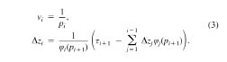
Here, ∆zi is the thickness of the ith layer, (i ≥ 0), vi is its velocity, and

is the intercept time per unit layer depth (with hi being the incidence angle in the ith layer) (Sheriff and Geldart, 1995, equation 4.42). The preceding parameters are computed in a single pass from the top of the model to its bottom, and the resulting model predicts all the travel times si(pi) exactly. Earth-flattening transformation can be applied if true velocities and depths are of interest; however, it is not required for the travel-time interpolation.
The resulting ∆z(p) parameterization possesses two important properties that make it particularly useful for the subsequent interpolation: (1) the values of ∆z(p) can be interpreted as layer thicknesses associated with the subsurface locations; (2) as differential characteristics of the travel times (compare the second equation 3), the values of ∆z(p) are computed progressively for decreasing values of p, and the shallower layers absorb the static time shifts. Consequently, the ∆z(p) parameterization is less sensitive to the propagation of near-source time shifts (caused by the variations in the crustal structure) across the entire offset range, which is the key problem with interpolation of travel times using a direct, t(r) parameterization (1).
The velocity model (3) is unique by construction, and it predicts each of the input first-arrival times s(p) accurately. To add lateral variability to these models, we associate (somewhat arbitrarily) each value of ∆z(p) with the location of the midpoint of the great arc on the surface along which this value of p was observed (Fig. 47). This results in a set of ∆z(p|xi,yi) values of layer thicknesses at different geographical locations.
Spatial Interpolation
In the last step of the travel-time-mapping procedure, for each p, the corresponding layer thicknesses ∆z(p|xi,yi) are interpolated into a dense, 2D surface grid by using minimum-curvature splines (adapted from Smith and Wessel, 1990), constrained to values of ∆z ≥ 0. The result is a continuous, 3D layer-thickness model ∆z(p,x,y) that reproduces the input data and is suitable for ray tracing, computation of SSSCs, plotting, and interpretation.
Thus, with complete travel-time curves from zero to the maximum recording offset available, the procedure represented by expression (2) results in an interpolated, 3D, travel-time model in a single pass, without uncertainties or iterative inversion steps. In this mode, this procedure could provide an alternative way to interpolate the regionalized travel times t(dSR) in equation (1). However, real travel-time data often have offset and travel-time gaps, and such gaps need to be accounted for in the interpolation. Clearly, no ideal solution exists to this problem of missing data, and we resort to a reasonable heuristic approach, based again on interpolation of the s(p) travel times.
Gaps in the Offset Coverage.
If offset gaps are present in the data, we repeat the described mapping several times. In the first pass, we initialize the ∆z(p) model by using a single reference travel-time curve that could be, for example, an average t(r) picked for the entire region. The exact shape of this starting dependence is not essential. Ray tracing within this model results in s(p) curves computed at the locations of the gaps in offset coverage. For each travel-time gap, predicted reference s(p) times are linearly scaled (also using a factor linearly varying in p) so that they fit within the gap (Fig. 48). After the gaps are filled, the interpolation is per- formed again, and this procedure is repeated iteratively. In our DSS data set, the resulting travel-time field converged in two iterations.
Other possible alternatives to the described s(p) interpolation procedure include linear interpolation across the gap in the t(x) or s(p) domains (Fig. 49). Our preferred interpolation approach leads to travel times that are intermediate between these two extremes and that also resemble the travel-time patterns recorded in the adjacent areas. Therefore, this approach appears to provide a reasonable approximation of the missing data within the offset gaps.
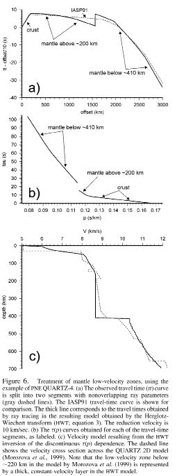
Gaps in Travel-Time curves. Gaps in the travel-time curves caused by low-velocity zones within the mantle represent another problem still not addressed in the existing regionalizated travel-time models (Bondár et al., 2001) yet critical for our study area (Figs. 50-52) (Mechie et al., 1993; Morozova et al., 1999) . From the PNE studies, gaps of up to ∼5 sec occur near ∼1500 km offsets (Fig. 46) from shots within the East European Platform and in the southern part of Western Siberia (Fig. 42) but not under the Siberian Craton (Mechie et al., 1997; Nielsen et al., 1999). To account for such gaps in the s − p interpolation method, it is only necessary to split the t(r) travel-time curves into the appropriate segments with nonoverlapping ray parameters (Fig. 50). This results in discontinuous s(p) dependencies (Fig. 51), with the corresponding ∆z(p) models (Fig. 52) reproducing the travel-time gaps (thick line in Fig. 52), and the travel-time interpolation providing smooth transitions into the areas where no gaps are found.
Low-velocity zones lead to strong nonuniqueness of 1D travel-time inversion (3), and additional constraints on the extents and amplitudes of the velocity anomalies are required (Bessonova et al., 1974; Morozov, 2004). In our modeling, low-velocity zones are replaced with depth intervals of zero vertical gradients (Fig. 52). Reflection travel times and amplitudes could be used to improve these models, but such data are limited to only a few interpretations (Morozova et al., 1999). Nevertheless, despite the uncertainty of the mantle structure, our travel-time modeling appears to reproduce the observed regional first-arrival travel times sufficiently closely (Fig. 50).
Prediction of Travel Times
The method was applied to each of the observed travel-time curves picked from 19 PNEs in northern Eurasia and from several published regional DSS investigations in Kazakhstan (Antonenko, 1984; Zunnunov, 1985; Shatsilov et al., 1993). To stabilize the interpolation near the edge of the model, and also to illustrate the use of generalized travel-time dependencies associated with tectonic types, additional travel-time curves were included within the Baltic Shield and East European Platform (Conrad et al., 2001) (Fig. 42). The resulting map, in the form of constant-slowness surfaces, z(p|x,y), is shown in Figures 53-55. Note that the principal objective of the ray-parameter parameterization is separation of the crustal (high values of p) and mantle (p ≤ 0.12 sec/km, that is, velocity greater than 8.3 km/sec) contributions. As expected, the high-p (small-offset) maps are based on denser data coverage and show more detail; at the same time, the sparsely sampled low-p readings still control the adjacent regions and no external reference model (such as the IASP91) is required. Note that for smaller regions (such as the Urals in Figs. 53-55), shallow (higher-p) structure appears to correlate with the regionalization, whereas at greater depths this correlation is less apparent.
To predict the travel times between any two points within the region (Figs. 53-55), we trace rays through the resulting ∆z(p|x,y) maps by using an approximate, 1.5D procedure corresponding to mapping (2). Travel times are computed within vertical cross sections along the great circle paths and assuming that the ∆z(p) layers are locally horizontal along the ray path (Fig. 56). With reference to the layer-stripping procedure (3), the predicted travel time t and offset r become:

and the summations are performed over all the N(p) layers for which pvi < 1. Because the layer thicknesses ∆zj(x,y) are now spatially variable, these summations are started from the source, proceed to the bottom layer, and go back to the surface near the receiver. The ray parameter p in expressions (5) is iteratively adjusted so that the ray ends at the receiver. Unlike two-point 3D ray tracing, this shooting method is fast and does not suffer from shadow zones caused by transitions across lateral- and depth-velocity contrasts.
When low-velocity zones are present, head waves from the shallow layers could mask the deeper arrivals in the first breaks (dashed line in Figs. 50-52). However, in practice, because of their low amplitudes, head waves are often not observed at large offsets, and travel-time gaps are identified in the first arrivals. To reproduce such travel-time gaps in ray tracing, head-wave propagation distances need to be restricted. In our approach, this is achieved by introducing an additional model parameter, α, controlling the maximum head-wave propagation distance:

where rcrit(p|x,y) is the critical distance for a ray with slowness p and bottoming beneath point (x,y). This parameter is also assigned to the individual travel-time curves and spatially interpolated together with ∆z. During ray tracing, the interpolated values of α are used to control the maximum extents of the head waves in each model layer (Fig. 57). In Figure 50 and in the following example, α was set constant and equal to 1.3 everywhere in the model.
Figure 34a shows the interpolated travel times for station Borovoye in Kazakhstan (BRVK) (Fig. 42) and surface sources within a radius of ∼2000 km around it, derived by using the 3D model in Figures 53-55. We subtracted the IASP91 times from the interpolated travel times, so that the resulting time differences can be directly compared with the SSSCs normally used in the travel-time calibration.
Discussion
The empirical travel-time-mapping scheme described by expression (2) should be viewed as an alternative travel-time interpolation scheme to method (1) rather than as an attempt to invert for the velocity structure within the region. This method still does not reflect the full complexity of the travel times (in particular, it does not account for their azimuthal dependence). Like any inversion of diving-wave travel times, the underlying model is highly nonunique (Morozov, 2004), and the choice of the HWT solution (3) is dictated by its smoothness, absence of negative-velocity gradients, and the ability to construct the model in a single pass of the algorithm. The only two objectives of this model are to accurately predict the observed first-arrival travel times while honoring the fundamental travel-time properties of body-wave seismic waves in the layered Earth. Note that within the context of these objectives, and because the preceding model uncertainty is not reflected in the first-arrival travel times, the HWT solution thus appears to be a good representative of the class of possible models.
Compared with the existing approach (1) (Bondár and Ryaboy, 1997), this method offers significant improvements in pursuing both of these objectives; first, by utilizing significantly larger and densely spaced travel-time data sets (both raw and derived from regional generalizations), and second, by emphasizing the offset dependence in the travel-time patterns. No regionalization (i.e., subdividing the area into blocks) is needed; however, the traditional regionalized travel times (Conrad et al., 2001) or velocity models could be used in this interpolation scheme along with other data, similarly to those for the Baltic Shield and East European Platform in Figures 53-55. Without the use of the DSS travel times and by assigning multiple sampling points and fixed travel-time curves within, for example, Conrad et al. (2001) regions, interpolation should also reproduce (not exactly but within the errors caused by the regions’ edge effects in formula 1) the predictions of this type of regionalization.
The resulting travel-time model of northern Eurasia (Figs. 53-55) reflects both the regional features and local variability sampled by the present data sets. The seismic velocity structure beneath this region differs from the global average, with the regional P waves at 2000 km arriving by ∼5 sec earlier than in the IASP91 model (Mechie et al., 1997) (Fig. 46). Within the region, significant structural variations are apparent (Fig. 46), suggesting that a single, 1D velocity model for the whole region (Ryberg et al., 1998) is hardly viable. By contrast, while retaining its character of a catalog of the observed travel times, the 3D model provides adequate representation of both the overall regional character of travel times and their local variability.
The SSSC surface obtained from the interpolated DSS travel times (Fig. 34a) illustrates the utility of the method for practical travel-time calibration. Although the number of data points used in the analysis is limited (Figs. 53-55), the SSSC reflects the key travel-time features of the region, such as the systematic P-wave travel-time advance relative to IASP91 (Fig. 34a). Note that the general pattern of the SSSC shows consistently increasing travel-time advances rather than concentric patterns typical of SSSCs derived by using the IASP91 travel times as the reference model (Yang et al., 2001). Such patterns arise from the tendency of conventional algorithms to revert to a reference model (such as IASP91) when no calibration data are available. By contrast, in our method, the average travel times in northern Eurasia are automatically accepted as the reference model, and the IASP91 model is not utilized at all.
The SSSC for BRVK (Fig. 34a) was derived without any GT events and also without any recordings at BRVK. Note that this SSSC correctly reproduces the regional travel-time trend and reduces the residuals of the events observed at the station (Fig. 34b). Accounting for the remaining residuals would clearly require detailed knowledge of the crustal structure or travel times from reliable events. This SSSC could thus be viewed as a reference model that could be further refined by using GT events. Implementation of 1.5D ray-tracing (Figs. 56-57) in a 3D ∆z(p|x,y) model cube is simpler than the travel-time interpolation across the boundaries of geographic regions (Bondár and Ryaboy, 1997; Bondár and North, 1999; Conrad et al., 2001), and it could be readily incorporated into SSSC modeling procedures.
To test the performance of our approximate SSSC, we subtracted its predicted travel times from the first-arrival times of 145 events recorded at BRVK from 1967 to 2000 (Conrad et al., 2001). Although obtained without using these events, the SSSC reflects the trend in their offset dependence (Fig. 34b); however, significant scatter is still present because of unresolved crustal and uppermost mantle variations and picking uncertainties. Unlike the apparent velocity variations, these factors should be more localized in space, and kriging (Myers and Schultz, 2000) could be used to spatially average and predict these residuals. However, we utilized a simpler technique consisting of a running average followed by interpolation utilizing the minimum-curvature splines (modified program surface from Generic Mapping Tools, Smith and Wessel, 1990). The resulting interpolated SSSC shows a somewhat stronger time advance relative to the IASP91 (Fig. 35a), with remaining travel-time residuals within ±1 sec (Fig. 35b). These residuals can be explained by neither source nor receiver travel-time delays and should be due to picking inconsistencies.
By introducing ray-parameter-dependent regionalization and mapping the travel times into depth, the new method also provides a link to model-based travel-time prediction techniques. However, instead of the true crustal and mantle velocities, it utilizes a 3D apparent velocity (ray parameter) model (Figs. 53-55) that is free from many uncertainties caused by the choice of inversion methods, regularization, and inherent ambiguity of the first-arrival inversion.
Transformation of the depth-interval model ∆z(p|x,y), into depth:

yields a 3D model of the apparent velocity structure of northern Eurasia (Figs. 58-61). Although bearing the typical ambiguities of first-arrival inversion (Morozov, 2004), the model still reflects the variations in the structure of the mantle in the region. The 3D travel-time modeling within this model should closely reproduce the observed first-arrival travel times; therefore, this velocity model could also serve as a reference for ray-tracing-based travel-time calibration and for generation of SSSCs. Compared with 3D travel-time tomography, the advantage of the proposed 1.5D method is in its natural handling of sparse travel-time data sets and inherent stability. No regularization, whose effects on the resulting velocity structure might be difficult to assess, is required. Because of its smooth character, the model is not likely to create problems for 3D ray tracing. Most importantly, in areas of poor data coverage, the resulting structure approaches a regional 1D model, and no reference or “preferred” model is required.
The described empirical travel-time calibration method contains potential for its improvement in several ways. Bayesian kriging could replace spline interpolation in predicting the spatial distributions of layer-thickness parameters ∆z(p|x,y), thereby providing statistical estimates of uncertainties in the apparent velocity models and travel times. Anisotropy parameters could be naturally incorporated in the model to account for azimuthal variations of the travel times. Because of the depth-ray-parameter parameterization (3), the method can utilize depth-velocity models (e.g., CRUST 5.1 in Mooney et al., 1998) that may be available for some locations in combinations with travel-time curves for other places. The travel-time models could be refined by incorporating detailed maps of the basement and Moho structure known from dense DSS and industry seismic studies (A. V. Egorkin, personal comm., 1995). Most importantly, this method could also be generalized to using, along with the DSS travel-time curves, much larger data sets of all available travel times recorded in the region. With these enhancements, the 3D apparent velocity parameterization scheme could combine the purely empirical, interpretative “regionalization” and the model-based tomographic methods into a common integrated framework required for CTBT monitoring.
Conclusions
Ray-parameter-dependent interpolation of the observed DSS first-arrival travel times results in a 3D apparent velocity model that could be utilized in travel-time calibration of northern Eurasia in several ways: (1) as a simple, purely empirical way to construct approximate SSSCs for any location within the region; (2) as a regionally variable 3D reference model that can be used for developing SSSCs; and (3) as an alternative way to perform travel-time interpolation in the existing empirical regionalization methods, with the advantage of utilizing the principles of model-based approaches. The key advantage of this method is in its ability of using large heterogeneous (travel- time, velocity) data sets with no classification or regionalization effort required. The resulting 3D model can be used to generate approximate SSSCs for any location, and mapping of the first-arrival travel-time patterns into depth leads to characterization of the general variability of the upper mantle velocity within the region.