The definition of electric current i is the time derivative of electric charge q, and, according to Faraday’s law voltage, v is the time derivative of magnetic flux ϕ. In 1971 Leon Chua noted that there ought to be six mathematical relations connecting pairs of the four fundamental circuit variables, i, v, q, and ϕ.1 In addition to the definition of electric current and Faraday’s law, three circuit elements connect pairs of the four circuit variables: resistance R is the rate of change of voltage with current  , capacitance C is the rate of change of charge with voltage
  and inductance L is the rate of change of magnetic flux with current
  . From symmetry arguments, Chua reasoned that there should be a fourth fundamental element, which he called a memristor (short for memory resistor) M, for a functional relation between charge and magnetic flux,
  .
.
In the case of linear elements in which M is a constant, memristance is identical to resistance. However, if M is itself a function of q yielding a nonlinear circuit element, then no combination of resistive, capacitive, and inductive circuit elements can duplicate the properties of a memristor. Almost 40 years after Chua’s proposal, memristor was found by scientists at HP Labs led by R. Stanley Williams.2,3 They suspected that memristive phenomenon has been hidden for so long because those interested were searching in the wrong places. Although the definition of memristor involves magnetic flux, magnetic field does not play an explicit role in the mechanism of memristance. As stated in their paper, the mathematics simply require there to be a nonlinear relationship between the integrals of the current and voltage [italics added]. The explicit relationship between such integrals based on the model by Strukov et. al. is detailed below.


Eq. (1) looks like Ohm’s law, but the generalized resistance R(x) depends upon the internal state x of the device. The time derivative of the internal state is a function of x and i. Strukov et. al. were the first to conceive a physical model in which x is simply proportional to charge q. They designed a device with R that can switch reversibly between a less conductive OFF state and a more conductive ON state, depending on x
The internal state x(t) is restricted in the interval [0, 1], when x(t) = 0, R = Roff and when x(t) = 1, R = Ron. The time derivative of x(t) is made to be proportional to current
in which the parameter β has a dimension of magnetic flux (in SI units, magnetic flux is measured in V s, or Wb). The HP scientists produced a semiconductor device to satisfy this condition, to be discussed shortly. Eq. (1) is rewritten as

Eliminating i(t) from Eq. (5) using Eq. (4), we can write the memristive system as a first-order differential equation of x(t). Defining the resistance ratio r = Roff/Ron, the equation becomes
Using ϕ = ∫ vdt and the property  , it is easy to integrate both sides
where c is a constant of integration determined by the initial value of x. This constant contains the past events of the input current i and plays an important role in a nonlinear system. Since x is proportional to charge, Eq. (7) indicates that the magnetic flux is a quadratic function of the charge, and the nonlinear relationship between the integrals of the current and voltage for a memristor is achieved.
The memristor invented at HP Labs is made of a thin film of titanium dioxide of thickness D sandwiched between two platinum contacts. The film has a region with a high concentration of dopants having low resistance Ron, and the remainder has a low dopant concentration and much higher resistance Roff. The application of an external bias v(t) across the device will move the boundary between the two regions by causing the charged dopants to drift. Let w(t) be the coordinate of the boundary between a less conductive OFF state and a more conductive ON state and μV the average ion mobility (measured in m2 s-1 V-1 in SI units), and Eq. (4) written in physical parameters is
which leads to
By comparing Eq. (4) and Eq. (8) we identify x = w/D and β = D2/μV . Recall that β has a dimension of magnetic flux, thus magnetic field is not directly involved in this memristor. Eq. (7), setting c to zero, becomes
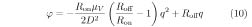
For Roff ≫ Ron, the memristance of this device is obtained
The q-dependent term is due to the nonlinear relationship between ϕ and q. For the first time, scientists wrote down a formula for the memristance of a device in terms of material and geometrical properties of the device. (An analogy is that for parallel plates, capacitance is expressed as C = ∊A/d2, where ∊, A, and d are permittivity, plate area, and plate separation, respectively. Similarly, resistance and inductance of devices can be expressed in terms of material and geometrical properties.) Because the coefficient of q is proportional to 1/D2, memristive behavior is increasingly relevant as electronic devices shrink to a width of a few nanometers. As semiconductor film of thickness D reduces from micrometer scale to nanometer scale, the nonlinear effect increases by a factor of 1,000,000.
As soon as researchers discovered the device, it was natural to measure the current responding to the applied voltage. If the applied voltage in Eq. (5) is
then replacing ϕ = ∫ v(t)dt with  cos(wt) in Eq. (7)
and using the quadratic formula to solve for x(t), we have
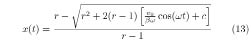
(We retain only the sign “-” in “±” so that the solution is in the interval [0, 1].) The current i(t) is proportional to the time derivative of x(t), which is
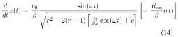
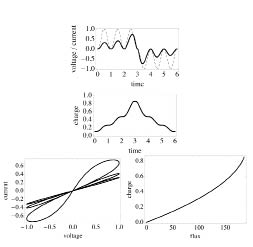
Our calculation shows that the current is the product of v(t) and a function of cos(wt). Important properties of a memristor can be understood from this expression. The current i(t) is zero whenever the the applied voltage v(t) is zero, regardless of the state x(t). Because the i–v curve must pass through the origin, the i–v Lissajous figure is double-loop curve—the most salient feature of the memristor. At high frequencies, cos(wt)/w under the radical sign becomes small, so the nonlinear contribution is suppressed. As a result, the i–v hysteresis collapses to a nearly straight line. These features are seen in Figure 301. The memory effect of a memristor is attributed to the constant of integration c that first appeared in Eq. (7). This constant cannot be removed by subtracting a constant from x(t) and remains after differentiating x(t) with time. Therefore, memristor response depends on history. As another example, with the applied voltage v(t) = ±v0 sin2(wt) shown in Figure 302, the solution is obtained by replacing ϕ = ±∫ v0 sin2(wt)dt = ±v0[t/2 - cos(wt) sin(wt)/(2w)]. We again see the “pinched loops” in the i–v plot. Strukov et. al. reported in their paper that i–v plots shown Figures 301 and 302 are regularly observed in their studies of titanium dioxide devices.
The most important lesson for students to learn from this note is that the familiar Ohm’s law v = iR is merely an approximation which is inadequate for a nonlinear circuit. Suppose that a scientist, who did not know the nature of the titanium dioxide device invented by the HP scientists, attempts to characterize this device on the i–v plane. If one treats the system as resistive, then based on Eqs. (12) and (14), the resistance would be
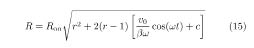
which is time-varying and frequency-dependent. In fact, such an erroneous interpretation of the i–v plot is the source of numerous confusions of “current-voltage anomalies” reported in unconventional elements. For a memristor, the constitutive relation is a curve in the q–ϕ plane, as depicted in Figures 301 and 302, expressed as a single-valued function of the charge q
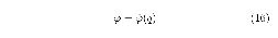
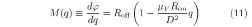
[This is a rather awkward notation to indicate that ϕ is a function of q.] Differentiating this equation with time results in
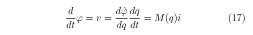
In terms of voltage and current, Eq. (16) assumes the form v = M(q)i. Because M(q) varies with the instantaneous value of charge, which bookkeeps the past events of the input current, it has a memory. Without recognizing this fact, it is difficult to use v = Ri to explain phenomena in nonlinear circuits properly. In retrospect, many “unusual hysteresis” in i–v plots of various circuits are actually due to memristance. With the model of Strukov et. al., a wide variety of eccentric and complex Lissajous figures that have been observed in many thin-film, two terminal devices can now be understood as memristive behavior. Such a concept is exceedingly useful in understanding hysteretic current-voltage behavior observed in nanoscale electronic devices and should be introduced to students as early as possible. It is worth mentioning that in preparing the paper for Nature, Dr. Williams and his colleagues were intentionally writing for curious undergraduates. Students are encouraged to read the original paper for further discussions and potential applications.
Figure 301: The charge and current of a memristor responding to the applied voltage v0 sin(wt) (dashed line in the v–t plot) based on Eqs. (13) and (14) are shown; the q–ϕ plot is made using Eq. (7). In these plots, voltage, current, time, magnetic flux, and charge are expressed in units of v0, v0/Ron, t0 ≡ β /v0, β and i0t0, respectively. The resistance ratio is r = Roff/Ron = 160; the dimensionless combination of v0/(βw) is set to be 100/∏ , and β (physically D2/μV in which D is the film thickness and μV the mobility) is chosen to be 10-2/Wb. The i–v plot is produced using the parametric plot procedure in graphing software. In the i–v plot, a high-frequency (10w) response is shown, which appears almost as a straight line.
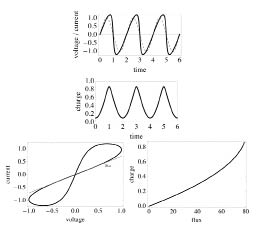
Figure 302: This figure is similar to Figure 2: the applied voltage is ±v0 sin2(wt) (dashed line in the v–t plot) and resistance ratio is Roff/Ron = 380. Notice that while i–v plot in this example appears to be complex, the pinched loops feature manifests itself vividly. Also the q–ϕ plot is simple: magnetic flux is a single-valued function of charge, see Eq. (7).